What would the data world be without SQL? And more importantly, what would business analysts, data analysts, and to a lesser extent, data engineers be without SQL? SQL is the lingua franca of data. It’s somewhat like English for international business. It’s an essential prerequisite.

What’s fascinating about SQL is that it’s a relatively easy language to learn. This explains why teams of analysts have quickly been established in companies of all sizes — large, medium, or small. People from diverse backgrounds, from engineering schools to business schools, often transition into data roles, which is made easier by how relatively simple it is to learn SQL.

A quick note: most business or data analysts primarily use the DQL (Data Query Language) part of SQL. The analyst’s job generally doesn’t involve access control, creating new tables, or records. All that’s needed is to select the necessary data for analysis, join or aggregate it in a useful way. Usually, writing SQL queries takes the least amount of time, as the real challenge lies in understanding business issues, identifying data sources, understanding them (which can be tough when there’s no documentation), evaluating data quality, and solving the problem at hand.

In most cases, the SQL queries you need to write are relatively simple. However, there are situations where things get a bit more complicated, where the structure of database tables requires advanced SQL features. These are the cases I will cover in this article. We’ll discuss joins, nested and repeated data, analytical functions, and how to write efficient queries. It’ll be a bit long, but it will be extremely useful for you if you want to become a SQL master. So grab your cup of coffee or tea (if you’re a tea person like me), and let’s dive in!

The Romantic World of Joins

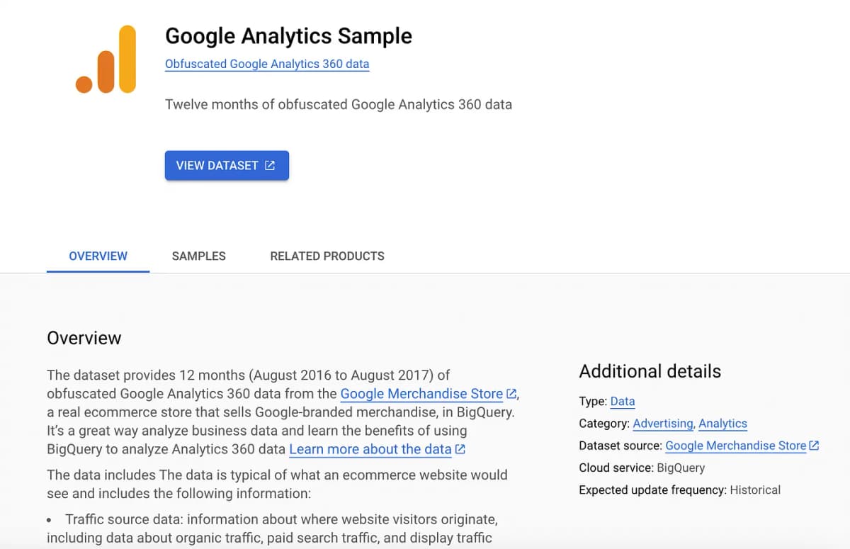
First of all, let me say this: there are many public datasets available online (Kaggle, BigQuery) if you want to practice your SQL skills. So don’t let that hold you back. I just spent a few minutes exploring the datasets available on BigQuery, and they are super interesting. I particularly liked this one and will probably focus on it later in this article series.

But enough digression. Let’s get back to business: joins.

The baseline level of data analysis in a company is Excel, sometimes with a bit of VBA for automation. But just because Excel is at this baseline doesn’t mean it’s less important or impactful than the tools in a modern data stack. Excel is fantastic when dealing with relatively small datasets. An Excel sheet can hold a maximum of 1,048,576 rows and 16,384 columns. Even reaching that point significantly degrades performance, making it slower and less productive. However, even in Excel, key concepts are present (tables, rows, columns, pivot tables, VLOOKUP or HLOOKUP for table cross-referencing, index creation). It may be basic, but the essentials are there.

The problem with Excel is that nothing is centralized. Everyone has their own file, edits it, potentially makes errors, calculates indicators in their own way, and it becomes too manual. The result is a lot of time spent compiling disparate data, trying to explain discrepancies in indicators, only to realize it was due to different methods of estimating parameters. Beyond that, when using Excel, you often need to cross-reference data from one sheet with data from another. This might involve creating an index, concatenating columns, trimming, etc., before reconciling. The SQL equivalent is joins.

SQL joins are essential. First, because the whole point of relational databases is to split data across multiple tables linked by secondary IDs or lookup tables. By design, this means that during analysis, you’ll need to join tables to restore the primary or secondary data in full. Secondly, joins are crucial because the most interesting analyses rarely concern just one table, but instead seek insights that emerge at the intersection, the join, or, if I may, the “marriage” of several tables.

Sometimes, tables are poorly designed or contain so many details and complex fields that splitting them and self-joining can be useful. So, not everything is always about linking to another table; sometimes, it’s about a self-referential link within a single table. There are several types of joins, with some more commonly used than others. The first is the “INNER JOIN.” Between two tables, A and B, linked by a secondary key, an INNER JOIN combines only the common elements between the two tables. For example, imagine you have access to a Clients table and an Orders table. The Orders table contains a reference (‘id_client’) linked to the client who placed the order.

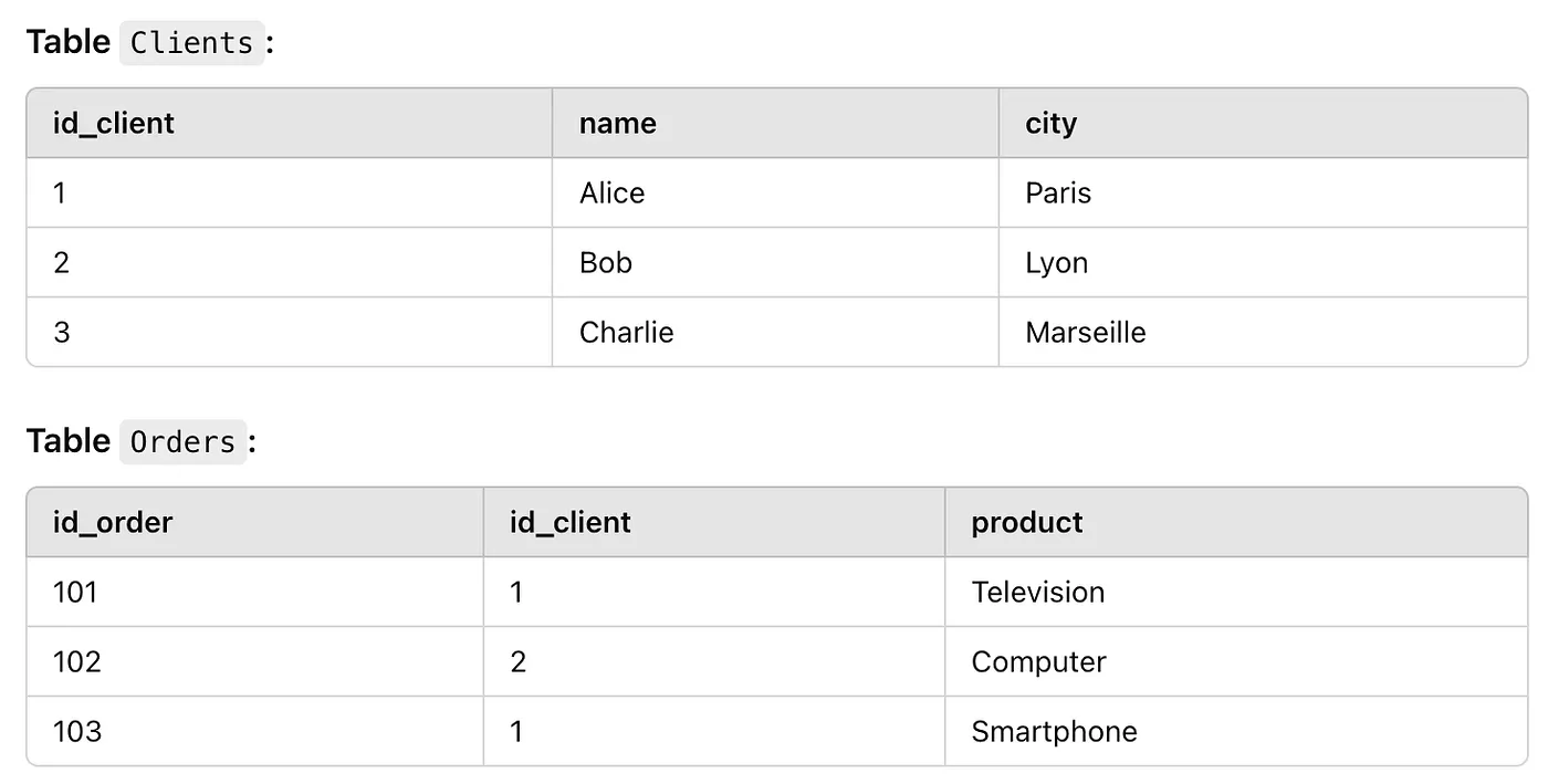
To find and return the list of orders along with client information, you’d perform an INNER JOIN between the Clients and Orders tables. The SQL query would look like this:

SELECT Clients.name, Clients.city, Orders.product
FROM Clients
INNER JOIN Orders
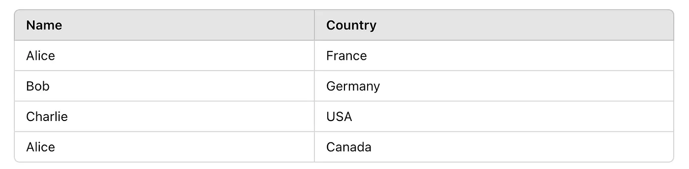
ON Clients.id_client = Orders.id_client;

The result will look like this:

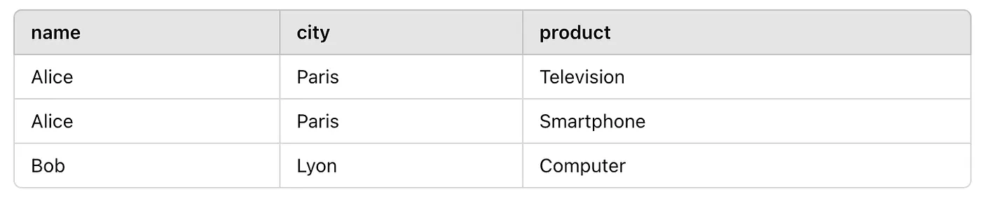
You’ll notice that there’s no mention of Charlie because Charlie doesn’t appear in either the Clients or Orders tables. Everything so far is quite basic and simple. I’ll cover more complex examples in the next articles in this series, but for now, it’s important to master the fundamentals.

Other frequently used joins include LEFT JOIN and RIGHT JOIN. A LEFT JOIN (or LEFT OUTER JOIN) returns all rows from the left table and the matching rows from the right table. If there’s no match, the right table columns will contain null values.

Here’s an example using our Clients and Orders tables:

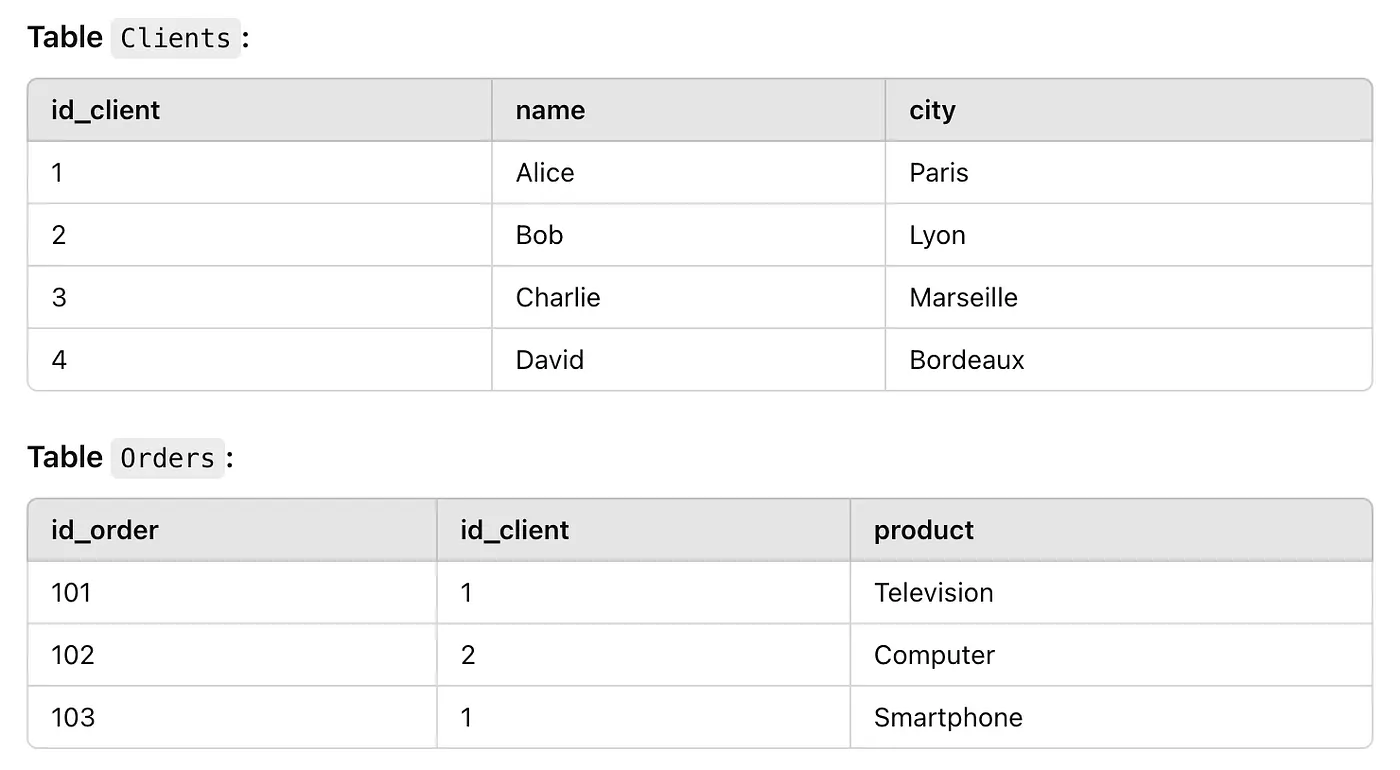
SELECT Clients.name, Clients.city, Orders.product
FROM Clients
LEFT JOIN Orders
ON Clients.id_client = Orders.id_client;

By performing a LEFT JOIN, all the clients present in the clients table will appear in the final table. For clients who have not placed any orders, the columns corresponding to the orders table will contain NULL values.

A RIGHT JOIN (or RIGHT OUTER JOIN) is similar to a LEFT JOIN, except it returns all rows from the right table (Orders), even if some don’t have a match in the left table (Clients).

SELECT Clients.name, Clients.city, Orders.product
FROM Clients
RIGHT JOIN Orders
ON Clients.id_client = Orders.id_client;

In practice, RIGHT JOIN is rarely used because any RIGHT JOIN can be easily rewritten as a LEFT JOIN by reversing the order of the tables.

Aside from the common join types (INNER JOIN, LEFT JOIN, RIGHT JOIN, FULL JOIN), there are other specific joins like UNION and UNION ALL. These aren’t technically “joins,” but they combine the results of multiple queries, which can be useful in advanced cases.

The UNION operator combines the results of two or more queries and removes duplicates. It’s useful when you want to merge result sets from separate tables or queries with the same structure (same number of columns and data types).

Here’s an example where we combine a list of European and American clients, removing duplicates:

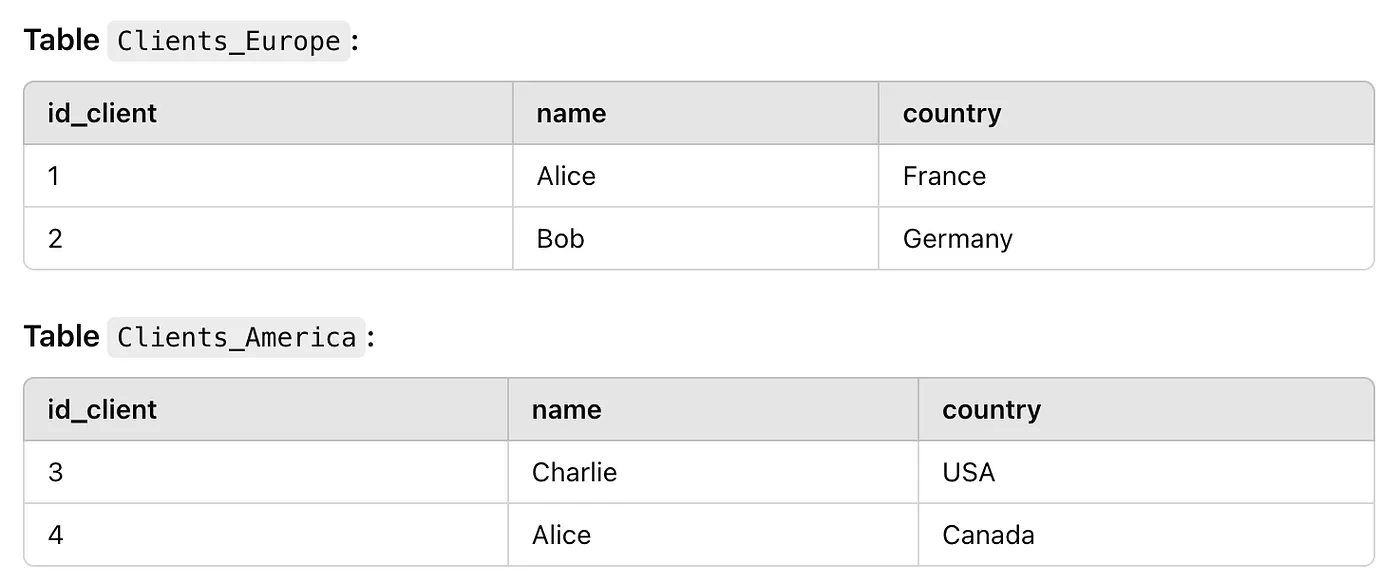
SELECT name, country FROM Clients_Europe
UNION
SELECT name, country FROM Clients_America;

In this case, UNION combines the results, removing duplicates. If Alice appears in both tables with the same details, she will only appear once in the result.

UNION ALL is similar but does not remove duplicates. It returns all rows from the combined queries, even if they are identical.

SELECT name, country FROM Clients_Europe
UNION ALL
SELECT name, country FROM Clients_America;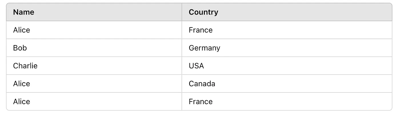

Other less common result combination operations include:

-EXCEPT: Returns rows present in the first query but absent from the second. This can help identify records unique to one table compared to another. -INTERSECT: Returns only rows that exist in both queries, helping find records common to two tables.

These methods require similar query structures (same column names and types). For example:

SELECT name, city FROM Clients
EXCEPT
SELECT name, city FROM Suppliers;

The truth is, in 99% of cases, you’ll mostly use LEFT JOIN. So, while it’s important to learn the other types of joins, focus on mastering LEFT JOIN.

We’ll revisit the Google Analytics public table example mentioned earlier to illustrate these concepts with more practical examples. The table is obfuscated, so don’t expect to perform highly detailed analyses, but we’ll use it for demonstration.

Exploiting this table requires using CTEs (Common Table Expressions), likely multiple ones. I assume you’re already familiar with CTEs, but if not, here’s a quick reminder.

A CTE is a temporary query you can define to simplify your SQL queries. It creates a temporary table available only during the query’s execution. CTEs are particularly useful for making complex queries more readable and reusable.

Here’s the classic syntax for a CTE:

WITH cte_name AS (
    SELECT column1, column2
    FROM table_name
    WHERE condition
)
SELECT *
FROM cte_name
WHERE another_condition;

Tip: CTEs are incredibly handy, and it’s recommended to use them often. While not strictly necessary, they greatly improve the readability of SQL queries, especially when they become long and complex. Structuring your code this way makes your logic easier to follow and debug.

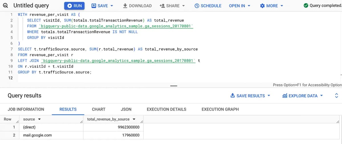
Here’s an example where we calculate total revenue by traffic source. We first calculate total revenue per visit (via a CTE) before aggregating by source.

Other CTE use cases include:

User Segmentation: Use a CTE to divide users into segments (e.g., new vs. returning users) and then compare their performance in terms of conversions or page views.

WITH user_segments AS (
    SELECT fullVisitorId, visitNumber,
           CASE WHEN visitNumber = 1 THEN 'New' ELSE 'Returning' END AS user_type
    FROM `bigquery-public-data.google_analytics_sample.ga_sessions_20170801`
)
SELECT user_type, COUNT(fullVisitorId) AS user_count
FROM user_segments
GROUP BY user_type;

Device Performance: Use a CTE to calculate engagement rates by device type, e.g., by analyzing page views or time spent on the site per mobile, desktop, etc.

WITH device_engagement AS (
    SELECT device.deviceCategory, AVG(totals.pageviews) AS avg_pageviews
    FROM `bigquery-public-data.google_analytics_sample.ga_sessions_20170801`
    WHERE totals.pageviews IS NOT NULL
    GROUP BY device.deviceCategory
)
SELECT d.deviceCategory, d.avg_pageviews
FROM device_engagement d;

Bounce Rate by Device: This query analyzes how many users leave the site after viewing just one page (bounce rate) and determines whether this rate differs by device type (mobile, desktop, tablet).

WITH bounce_rate AS (
    SELECT device.deviceCategory, COUNT(visitId) AS total_bounces
    FROM `bigquery-public-data.google_analytics_sample.ga_sessions_20170801`
    WHERE totals.bounces = 1
    GROUP BY device.deviceCategory
)
SELECT b.deviceCategory, b.total_bounces, t.trafficSource.source
FROM bounce_rate b
LEFT JOIN `bigquery-public-data.google_analytics_sample.ga_sessions_20170801` t
ON b.deviceCategory = t.device.deviceCategory

Geographical User Analysis: This query helps businesses understand where their visitors are coming from geographically, enabling them to target specific regions with localized marketing efforts.

WITH geo_summary AS (
    SELECT geoNetwork.country, COUNT(visitId) AS total_visitors
    FROM `bigquery-public-data.google_analytics_sample.ga_sessions_20170801`
    GROUP BY geoNetwork.country
)
SELECT g.country, g.total_visitors, t.trafficSource.source, t.device.deviceCategory
FROM geo_summary g
LEFT JOIN `bigquery-public-data.google_analytics_sample.ga_sessions_20170801` t
ON g.country = t.geoNetwork.country
LIMIT 100;

As you can see from the above examples, many of the queries you’ll write in a business context involve using a CTE, followed by joins (typically LEFT JOIN between two or three tables), filters (with WHERE or HAVING), groupings (via GROUP BY), and aggregations (such as AVG, COUNT, SUM).

These elements are key to extracting meaningful, actionable insights from large datasets. For example, you may need to calculate the performance of a marketing campaign based on traffic, conversion rates, or revenue generated by source and device.

Let’s end with a complete example.

Here’s a query that analyzes revenue by device type and traffic source while filtering the results to include only visits that generated transactions:

WITH revenue_by_device_and_source AS (
    SELECT
        device.deviceCategory,
        trafficSource.source,
        SUM(totals.totalTransactionRevenue) AS total_revenue
    FROM
        `bigquery-public-data.google_analytics_sample.ga_sessions_20170801`
    WHERE
        totals.totalTransactionRevenue IS NOT NULL
    GROUP BY
        device.deviceCategory, trafficSource.source
)
SELECT
    r.deviceCategory,
    r.source,
    r.total_revenue,
    COUNT(t.visitId) AS total_visits
FROM
    revenue_by_device_and_source r
LEFT JOIN
    `bigquery-public-data.google_analytics_sample.ga_sessions_20170801` t
ON
    r.deviceCategory = t.device.deviceCategory
    AND r.source = t.trafficSource.source
GROUP BY
    r.deviceCategory, r.source, r.total_revenue
HAVING
    r.total_revenue > 0
ORDER BY
    r.total_revenue DESC;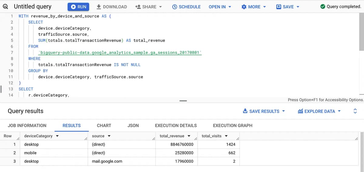

This query helps understand which devices (mobile, desktop, etc.) and traffic sources (Google, Direct, Social, etc.) generate the most revenue. This insight enables businesses to allocate marketing resources more efficiently, optimize the user experience on key devices, and focus on the most profitable traffic sources.

This is an excellent example of how to use CTEs, joins, aggregations, and groupings in business analysis.

But we’re just scratching the surface. In the next article in this series, we’ll dive even deeper, exploring powerful analytical functions like FIRST_VALUE(), LEAD(), LAG(), RANK(), and the OVER clause. These are essential tools for advanced SQL analyses, particularly useful when you want to:

-Analyze trends over time: For example, see how an indicator evolves from one row to another with LAG() or LEAD().

-Extract information relative to a position in a dataset, such as identifying the first value with FIRST_VALUE() or ranking elements using RANK().

-Work on data windows using the OVER clause, which allows partitioning data and performing calculations on subsets, all within the same query.

These functions will enable you to analyze data much more fluidly and granularly, especially when dealing with time series, rankings, or comparisons between successive records.

In the next article, we’ll go through concrete examples illustrating how these functions can transform datasets into actionable insights for business decision-making. Get ready to unlock the full potential of analytical functions for even more powerful SQL analyses!